Long gone are the days where spreadsheets were exclusively the domain of tweed-wearing accountants with horn-rimmed glasses in musty basements and beige cubicles. Today, spreadsheets are identified as a game-changing tool across hundreds of domains, some of them incredibly inapt!
But rather than explain why you shouldn’t, as the British Government tried to do, use Excel to store massive amounts of Covid data, I’m going to teach you how to use Excel better.
Note: I’m referring to Excel here, but other spreadsheet software should have largely the same functionality.
Excel is strong and so can you
Excel is powerful, but most users only wield a tiny fraction of its power. The more you wield, the more Excel can do, and, in a perfect world, the less you have to do by hand. Learn more, work less.
I believe there are ten steps you can take in Excel. Ten skills you can master that each represent a “leveling up”, a key shift in your understanding of the power of Excel.
Will mastering these 10 skills teach you everything about Excel? No! They’ll probably teach you less than 30% of the tools Excel provides and the power it contains. But each one will enable you to accomplish way more, and will represent a broader set of skills.
The list
Each of these ten levels is presented as a base skill, with opportunities to take it a step further. I have arranged these from most basic to most complex. The first few levels are things I would expect every Excel user to know, while the last few I would expect to be relegated to the domains of experts.
Remember, we’re all born knowing nothing, and the first time you learn even the most basic of features can save hours of work.
Note: This is not intended to be a tutorial, but to make you broadly aware of what tools are available. I will be linking to other resources throughout, and only explaining in detail where I deem it prudent.
1. Basic formulas
Open a cell, type =a1+b1 and watch the numbers dance and change before you. Everything updates in real time, and you can reference other cells. It’s magic!
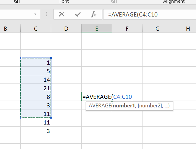
Get more complex with things like =sum(a1:a50) or =average(b1:b500). Even better, stop typing cell references by hand: after your opening ( parenthesis, cell the cell or drag over a range to fill it in for you.

Take formulas a step further
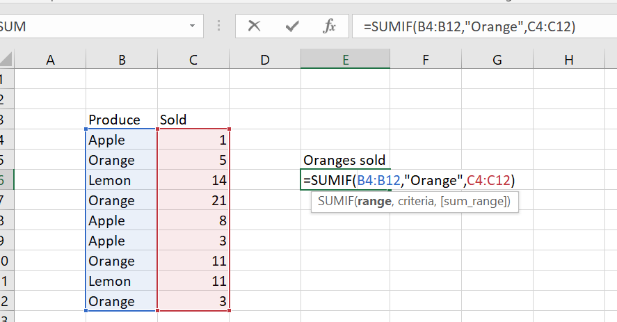
Use more advanced formulas like counta(a1:a500) to get a count of how many cells are not empty, or sumif() and countif() to count or sum cells based on various criteria. Things like “How many oranges did I sell”?

Take it another step further
You can even nest equations. Ask questions like what’s the average of the sum of each month? Or take the sum of the maximum value of each month’s sales =sum(max(a1:a12), max(b1:12),max(c1:c12)).
Learn your basic formulas like round(), min(), and max() and combine them in powerful ways.
Note: Not comfortable with long formulas yet? Use an intermediary cell. Make G20 the max of a1:a12, and then reference G20 elsewhere. Nesting keeps your logic in one place, and stops your spreadsheet from getting cluttered. But you don’t have to learn everything in one step! Progress comes in pieces.
2. Fill tool (ctrl+d)
So you’ve written a formula. Maybe you’ve got a few columns of data and you need to combine it. Maybe you need C1 to contain the value of A1*B1. Easy enough. =A1*B1. Oh, what’s this? You need the same thing in C2? Okay, copy, paste, change it to =A2*C2*. Woof! This is going to get tedious!
Surely, there’s an easier way?
There is! The fill tool! Simply enter your formula in once, then put your cursor over the bottom-right cell and drag down. Voila! Excel adjusts your formulas for you!
Even better, you can also drag the handle to the right (if you’re filling rows instead of columns), or use ctrl+D to fill down (and ctrl+R to fill to the right).
No more manually copying and editing formulas by hand!
3. Conditional formatting
Need to see what’s going on at a glance? Conditional formatting lets you automatically color cells based on certain rules.
This is useful for things like:
- Color all cells with a negative value red
- Show me the biggest / smallest values in this column
- Set up a gradient so the biggest values are green and the smallest are red
- Set up a gradient from red (very negative) to green (very positive) to see how these values compare to the average
Take formats a step further
You can set up formatting based on an equation (such as comparing against a value in a specific cell, or the average of a column). You can also base the entire formula off of another cell entirely.
Bonus: the format painter
If you’ve styled a cell the way you want (bolded, font size, borders, color, what have you), you can easily copy it to another cell with the format painter. Simply click the styled cell, click the painter, then click the cell you want to style.
Want to style a whole bunch of cells? Drag it over a range, or double-click the format painter to put it in “sticky” mode.
This is also useful if you’ve told a cell to be formatted as currency, or a number, or as text.
Tip: If you’re going to be entering things that excel might confuse for another format (like
+1or4-1orapr5), you can either format the cell as text, or type a ' before your data.
4. Sort and filter
If you’ve got a lot of data, you might find it useful to only look at a specific subset of it. Sort and filter features are extremely powerful, and fairly self-explanatory.
You can set up multiple layers of sort, so you are sorting first by country, then by state, then by last name, for example. Filtering can be applied to every column, allowing for a structured slice of your data.

5. Learn the : notation
It’s useful to reference a range by using the starting and ending cells. a1:a5 refers to a1, a2, a3, a4, and a5.
But you can also have 2D ranges. a1:b2 includes a1, b1, a2, and b2.
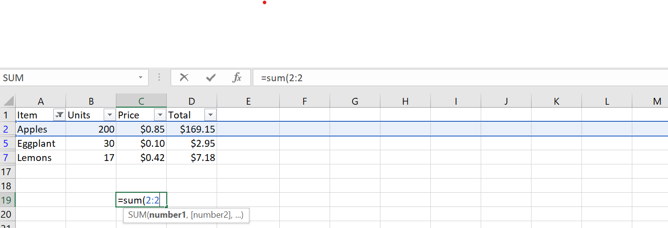
Taking it a step further, you can reference entire columns (a:a) or entire rows (1:1)

So while you can do =sum(a1, a2, a3), it’s faster and easier to just do =sum(a1:a3). With column and row references, you no longer need to guess how many entries exist. Instead of doing =average(a1:a500) and hoping you remember to update your formula when that 501st piece of data comes in, simply use =sum(a:a) and rest without worry.
More to come
That’s all for part 1. Join us next week for part 2, where we cover conditionals, pivot tables, and other advanced techniques.
If you’ve mastered these first 5 levels, you’re a proficient and probably competent Excel user. If you master the next five, you’re flirting with expertise and mastery.
But even those tricks won’t make you ready for the big time.
Disclaimer: at the time of this writing, I am employed by Microsoft, and have worked on Excel. These opinions are my own, and are not endorsed by my employer.
